A tutorial on the free-energy framework for modelling perception and learning
Based on K. Friston and following R. Bogacz I shortly summarise the former, and solve the programming exercises given in the paper.
Why is this important/exciting?
R. Bogacz delivers a detailed and beautifully made tutorial on a subject that can be very difficult to understand, Variational Bayes, as seen from Karl Fristons perspective; Namely invoking the Free-Energy principle to motivate Active Inference. In the last decade, Active Inference has gained traction with the wider neuroscientific community, and recently Karl was measured to be the most influential neuroscientist in the modern era.
Nomenclature:
I use the same notation as in R. Bogacz. The code implements and refers to equations in the paper, and network graphs were provided by Bogacz himself.
Introduction - Biological intuition
A simple organism is trying to infer the size \(v\) of a food item. The only source of noisy information is one photoreceptor that signals the light reflected from this item, we denote this \(u\). The non-linear function that relates size \(v\) to photosensory input \(u\) is assumed to be \(g(v)=v^2\). We assume that this signal is normally distributed with mean \(g(v)\) and variance \(\Sigma_{v}\).
Part I - Bayes
We can write of the the likelihood function (probability of a size \(v\) given a signal \(u\)) as
\[p(v\vert u)=f(u;g(v),\Sigma_{u})\]where
\[f(x;\mu,\Sigma)=\frac{1}{\sqrt{2\pi\Sigma}}\mbox{exp}\left(-\frac{(x-\mu)^{2}}{2\Sigma}\right)\]is the normal distribution with mean \(\mu\) and variance \(\Sigma\).
Through learning or evolutionary filtering, the agent has been endowed with priors on the expected size of food items, and therefore expects sizes of food items to normally distributed with mean \(v_{p}\) and \(\Sigma_{p}\) where the subscript \(p\) stands for prior. Formally
\(p(v)=f(v;v{p},\Sigma_{p})\).
To compute the exact distribution of sensory input \(u\) we can formulate the posterior using Bayes theorem
\[p(v|u)=\frac{p(v)p(u|v)}{p(u)}\]where the denominator is
\[p(u)=\int p(v)p(u|v)dv\]and sum the whole range of possible sizes.
The following code implements such an exact solution and plots it.
import numpy as np
import seaborn as sns
import matplotlib.pyplot as plt
from scipy.stats import norm

sns.set(style="white", palette="muted", color_codes=True)

%matplotlib inline
# non-linear transformation of size to perceived sensory input e.g. g(phi)
def sensory_transform(input):

    sensory_output = np.square(input)

    return sensory_output
The reason we explicitly define \(g(\cdot)\) is that we might want to change it later. For now we assume a simple non-linear relation \(g(v)=v^2\). The following snippet of code assumes values of \(v,\Sigma_u,v_p,\Sigma_p\) and plots the posterior distribution.
def exact_bayes():

    # variabels
    v = 2 # real size of item
    sigma_u = 1 # standard deviation of noisy input
    v_p = 3 # mean of prior
    sigma_p = 1 # variance of prior / sensory noise
    s_range = np.arange(0.01,5,0.01) # range of sensory input
    s_step = 0.01 # step size

    # exact bayes (equation 4)
    numerator = (np.multiply(norm.pdf(s_range,v_p,sigma_p),# prior
                            norm.pdf(v,sensory_transform(s_range),sigma_u))) # likelihood
    normalisation = np.sum(numerator*s_step) # denominator / model evidence / p(noisy input) (equation 5)
    posterior = numerator / normalisation # posterior

    # plot exact bayes
    plt.figure(figsize=(7.5,2.5))
    plt.plot(s_range,posterior)
    plt.ylabel(r' $p(v | u)$')
    sns.despine()
exact_bayes()
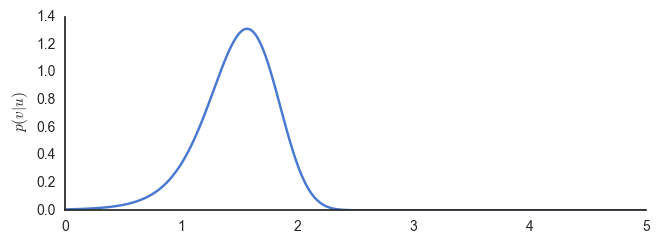
Inspecting the graph, we find that approximately \(\phi=1.6\) maximises the posterior. There are two fundamental problems with this approach
-
The posterior does not take a standard form, and is thus described by (potentially) infinitely many moments, instead of just simple sufficient statistics, such as the mean and the variance of a gaussian.
-
The normalisation term that sits in the numerator of Bayes formula
can be complicated and numerical solutions often rely on computationally intense algorithms, such as the Expectation-Maximisation algorithm.
Part II - Iteration using Eulers method
We are interested in a more general way of finding the value that maximises the posterior \(\phi\). This involves maximising the numerator of Bayes equation. As this is independent of the denominator and therefore maximising \(p(v)p(u\vert v)\) will maximise the posterior. By taking the logarithm to the numerator we get
\[F=\mbox{ln}p(\phi)+\mbox{ln}p(u|\phi)\]and the dynamics can be derived (see notes) to be
\[\dot{\phi}=\frac{v_{p}-\phi}{\Sigma_{p}}+\frac{u-g(\phi)}{\Sigma_{u}}g^{'}(\phi)\]The next snippit of code asumes values for \(v,\sigma_u,v_p,\sigma_p\) and implements the above dynamics to find the value of \(\phi\) that maximises the posterior using a manual implementation of the dynamics and iterating using Eulers method.
def simple_dyn():

    # variabels
    v = 2 # real size of item
    sigma_u = 1 # standard deviation of noisy input
    v_p = 3 # mean of prior
    sigma_p = 1 # variance of prior / sensory noise
    s_range = np.arange(0.01,5,0.01) # range of sensory input
    s_step = 0.01 # step size

    # assume that phi maximises the posterior
    phi = np.zeros(np.size(s_range))

    # use Eulers method to find the most likely value of phi
    for i in range(1,len(s_range)):

        phi[0] = v_p
        phi[i] = phi[i - 1] + s_step * ( ( (v_p - phi[i - 1]) / sigma_u ) +
        ( ( v - sensory_transform(phi[i - 1]) ) / sigma_u ) * (2 * phi[i - 1]) ) # equation 12

    # plot convergence
    plt.figure(figsize=(5,2.5))
    plt.plot(s_range,phi)
    plt.xlabel('Time')
    plt.ylabel(r' $\phi$')
    sns.despine()
simple_dyn()

It is clear that the output converges rapidly to \(\phi=1.6\), the value that maximises the posterior.
So we ask the question: What does a minimal and biologically plausible network model that can do such calculations look like?
Part III - Biological plausibility
Firstly, we must specify what exactly biologically plausible means.
-
A neuron only performs computations on the input it is given, weighted by its synaptic weights.
-
Synaptic plasticity of one neuron, is only based on the activity of pre-synaptic and post-synaptic activity connecting to that neuron.
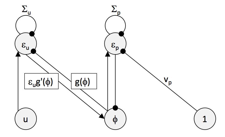
Consider the dynamics of a simple network that relies on just two neurons and is coherent with the above requirements of local computation
\[\dot{\epsilon_{p}} = \phi-v_{p}-\Sigma_{p}\epsilon_{p}\] \[\dot{\epsilon_{u}} = u-h(\phi)-\Sigma_{s}\epsilon_{s}\]where \(\epsilon_{p}\) and \(\epsilon_{s}\) are the prediction errors
\[\epsilon_{p} = \frac{v_{p}-\phi}{\Sigma_{p}}\] \[\epsilon_{s} = \frac{s-g(\phi)}{\Sigma_{s}}\]that arise from the assumption that the input is normally distributed (again, see Bogaez for derivations).
Below the network dynamics are sketched. Arrows denote excitatory input, circles inhibitory input, and unless specified (\(\theta,v_p,\Sigma_u,\Sigma_p\)), weights of connections are assumed to be one.
The next snippit of code implements those dynamics and thus, the network “learns” what value of \(\phi\) that maximises the posterior.
def learn_phi():

    # variabels
    v = 2 # real size of item
    sigma_u = 1 # standard deviation of noisy input
    v_p = 3 # mean of prior
    sigma_p = 1 # variance of prior / sensory noise
    s_range = np.arange(0.01,5,0.01) # range of sensory input
    s_step = 0.01 # step size

    # preallocate
    phi = np.zeros(np.size(s_range))
    epsilon_e = np.zeros(np.size(s_range))
    epsilon_s = np.zeros(np.size(s_range))

    # dynamics of prediction errors for size (epsilon_v) and sensory input (epsilon_u)
    for i in range(1,len(s_range)):

        phi[0] = v_p # initialise best guess (prior) of size
        epsilon_e[0] = 0 # initialise prediction error for size
        epsilon_s[0] = 0 # initialise prediction error for sensory input

        phi[i] = phi[i-1] + s_step*( -epsilon_e[i-1] + epsilon_s[i-1] * ( 2*(phi[i-1]) ) ) # equation 12
        epsilon_e[i] = epsilon_e[i-1] + s_step*( phi[i-1] - v_p - sigma_u * epsilon_e[i-1] ) # equation 13
        epsilon_s[i] = epsilon_s[i-1] + s_step*( v - sensory_transform(phi[i-1]) - sigma_p * epsilon_s[i-1] ) # equation 14

    # plot network dynamics
    plt.figure(figsize=(5,2.5))
    plt.plot(s_range,phi)
    plt.plot(s_range,epsilon_e)
    plt.plot(s_range,epsilon_s)
    plt.ylabel('Activity')
    sns.despine()
learn_phi()
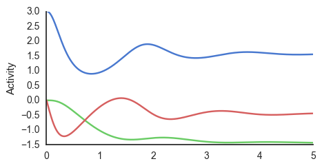
As the figure shows, the network learns \(\phi\) but is slower in converging than when using Eulers method, as the model relies on several other nodes that are inhibits and excites each other, which causes oscillatory behaviour. Both \(\epsilon_p\) and \(\epsilon_v\) oscillate and converge to the values where
\[\epsilon_{p} \approx 0\] \[\epsilon_{s} \approx 0.\]Which can be understood as the steady-state of the network. This means that minimising prediction errors (by learning the correct parameters) minimises the free energy potential - a tenet in Active Inference.
Part IV - Approximate estimation of \(\Sigma\)
Recall that we assumed that size \(v\) was communicated via. a noisy signal \(u\) assumed to be normally distributed. Above, we outlined a simple sample method for finding the mean value \(\phi\) that maximises the posterior \(p(v\vert s)\).
By expanding this simple model, we can esimate the variance \(\Sigma\) of the normal distribution as well. Considering computation in one single node computing prediction error
\[\epsilon_{i}=\frac{\phi_{i}-g(\phi_{i+1})}{\Sigma_{i}}\]where \(\Sigma_{i}=\left\langle (\phi_{i}-g_{i}(\phi_{i+1})^{2}\right\rangle\) is the variance of the best guess of \(v\), \(\phi_{i}\). Estimation of \(\Sigma\) can be achieved by adding a interneuron \(e_{i}\) which is connected to the prediction error node, and receives input from this via the connection with weight encoding \(\Sigma_{i}\), such as sketched in the figure below.
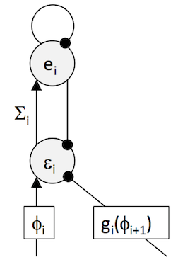
The dynamics are described by
\[\dot{\epsilon_{i}} = \phi_{i}-g(\phi_{i+1})-e_{i}\] \[\dot{e} = \Sigma_{i}\epsilon_{i}-e_{i}\]which the following snippit of code implements.
def learn_sigma():

    # variabels
    v = 2 # observed homeostatic error
    sigma_u = 1 # standard deviation of the homeostatic error
    v_p = 3 # mean of prior homeostatic error / noisy input / simple prior
    sigma_p = 1 # variance of prior / sensory noise
    s_range = np.arange(0.01,5,0.01) # range of sensory input
    s_step = 0.01 # step size

    # new variabels
    maxt = 20 # maximum number of iterations
    trials = 2000 # of trials
    epi_length = 20 # length of episode
    alpha = 0.01 # learning rate

    mean_phi = 5 # the average value that maximises the posterior
    sigma_phi = 2 # the variance of phi
    last_phi = 5 # the last observed phi

    # preallocate
    sigma = np.zeros(trials)
    error = np.zeros(trials)
    e = np.zeros(trials)

    sigma[0] = 1 # initialise sigma in 1

    for j in range(1,trials):

        error[0] = 0 # initialise error in zero
        e[0] = 0 # initialise interneuron e in zero
        phi = np.random.normal(5, np.sqrt(2), 1) # draw a new phi every round

        for i in range(1,2000):

            error[i] = error[i-1] + s_step*(phi-last_phi-e[i-1]) # equation 59
            e[i] = e[i-1] + s_step*(sigma[j-1]*error[i-1]-e[i-1]) # equation 60

        sigma[j] = sigma[j-1] + alpha*(error[-1]*e[-1]-1) # synaptic weight (Sigma) update

    # plot dynamics of Sigma
    plt.figure(figsize=(5,2.5))
    plt.plot(sigma)
    plt.xlabel('Time')
    plt.ylabel(r' $\Sigma$')
    sns.despine()
learn_sigma()
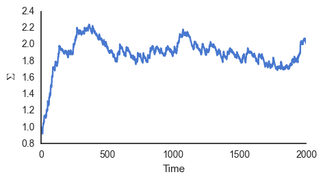
Because \(\phi\) is constantly varying phi = np.random.normal(5, np.sqrt(2), 1) \(\Sigma\) never converge to just one value, but instead to approximately 2, the variance of \(\phi_i\).