Non-ergodicity in a simple coin game
Based on a seminal talk by Ole Peters, I illustrate the fundamental difference between an ergodic and non-ergodic process using a simple coin game.
(If you download this notebook, you can use the interactive widgets to explore this yourself)
Why is this important/exciting:
In the talk I’ve linked to above, Ole Peters does a very good job at revisiting the properties of a mathmatical quantity (the ensemble average, or expectation operator) in the light of a novel understanding of dynamics. This question is fundamentally the same that motivated the St. Petersbrug Paradox and Daniel Bernoullis formulation of expected utility, that still lies as the foundation of all modern macro and micro economics.
In the following I will illustrate the essence of Peters talk, using a very simple coin game. The question we’re trying to answer is: Is this gamble worth taking?.
Dynamics:
- At each time step a fair coin is flipped and lands either heads or tails.
- For heads wealth increases with 50% e.g. \(W_t\cdot1.5\)
- For tails wealth decreases by 40% e.g. \(W_t\cdot0.6\)
Nonclamenture:
- \(W_t\) is the wealth at time \(t\) (
W_) - \(\mathbb{E}\) is the large-N limit expectation average (
E_) - \(\mathcal{A}\) is the the finite-time average (
A_) - \(\mu\) is the finite-ensemble mean (
mu)
Simulations:
import numpy as np
import matplotlib.pyplot as plt
import seaborn as sns

from ipywidgets import interact, interactive, fixed
import ipywidgets as widgets

sns.set(style="white", palette="deep", color_codes=True)

%matplotlib inline
def multiplicativeW(T, N, W, E, A, mu):

    w0 = 1 # start wealth
    c1 = 0.5 # multiplicative factor at win
    c2 = -0.4 # multiplicative factor at loss

    np.random.seed(1) # seeds numpy

    # preallocate
    c_ = np.empty((N,T))
    W_ = np.empty((N,T))
    mu_ = np.empty((T))
    E_ = np.empty((T))
    A_ = np.empty((T))

    for j in range(N):

        W_[j,0] = w0
        mu_[0] = w0

        for k in range(1,T):

            # coin dynamics
            c_ = np.random.choice([c1,c2])

            # wealth dynamics
            W_[j,k] = W_[j,k-1] * (1+c_)

            # empirical mean
            mu_[k] = np.mean(W_[:,k]) # finite ensemble mean

    # theoretical constants
    E_[0:T] = np.power(1+((0.5*c1)+(0.5*c2)),np.arange(0,T)) # expectation operator
    A_[0:T] = np.power(np.exp((np.log(1+c1)+np.log(1+c2))/2),np.arange(0,T)) # finite time-average

    # plotting
    fig = plt.figure(figsize=(12,5))
    plt.yscale('log', nonposy='clip')

    NUM_COLORS = N
    cm = sns.cubehelix_palette(8, start=10, rot=-.75,as_cmap = True)

    ax1 = fig.add_subplot(1,1,1)
    ax1.set_color_cycle([cm(1.*i/NUM_COLORS) for i in range(NUM_COLORS)])

    if W is True:

        for j in range(N):
            ax1.plot(W_[j],linewidth = 1)

    if E is True:
        ax1.plot(E_,linewidth = 2,color='k',label = (r'$\mathbb{E}$'))
        plt.legend(loc='upper left', fontsize=14)

    if A is True:
        ax1.plot(A_,linewidth = 2,color='r', label = (r'$\mathcal{A}$'))
        plt.legend(loc='upper left', fontsize=14)

    if mu is True:
        ax1.plot(mu_,linewidth = 2,color='r', label = (r'$\mu$'))
        plt.legend(loc='upper left', fontsize=14)
First, let’s assume that we play the coin game once every minute for an hour and plot just one (\(N=1\)) trajectory of the dynamic outlined above for \(T=60\) time periods.
interact(multiplicativeW, T = 60, N = 1, W = True, E = False, A = False, mu = False)
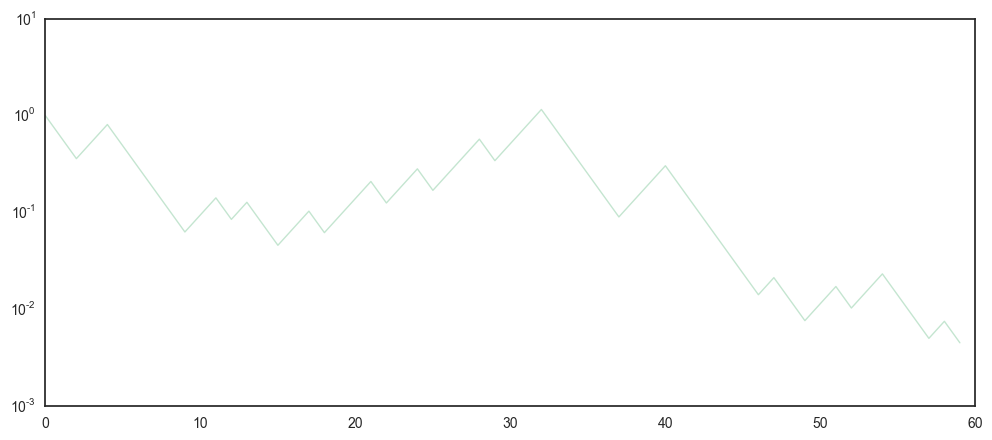
Its clear that this process got close to zero \((10^{-2})\) quite quickly (after 50 flips). However, it’s also quite noisy and difficult to make out, if this one trajectory was just a bit unfortunate. Lets repeat the game 100 times \((N=100)\) and see what happens.
interact(multiplicativeW, T = 60, N = 100, W = True, E = False, A = False, mu = False)
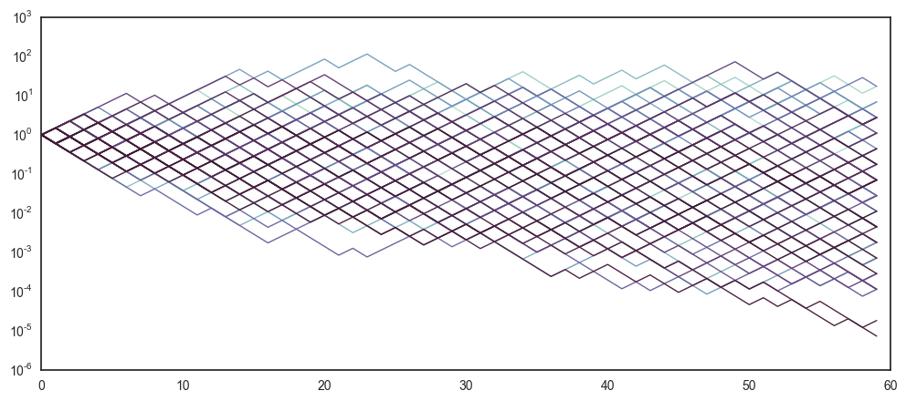
We’re still not getting much smarter. Looks like half on the trajectories are increasing, while the other half are dereasing - but it remains difficult to tell if this game is really beneficial.
To get rid of some of the noise, let’s try to average the 100 different trajectories.
interact(multiplicativeW, T = 60, N = 100, W = False, E = False, A = False, mu = True)
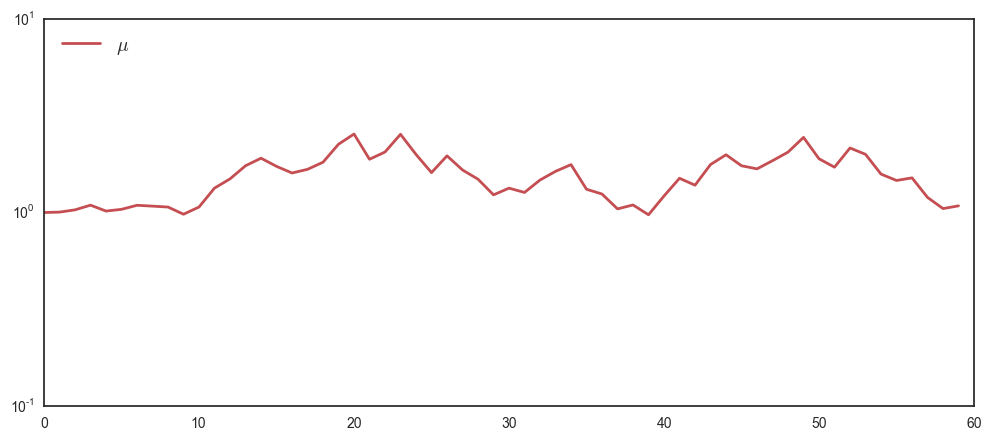
Which looks noisy around zero. To reduce the noise in the average, increase the number of plays to a large number, say \(N=10000\).
interact(multiplicativeW, T = 60, N = 10000, W = False, E = False, A = False, mu = True)
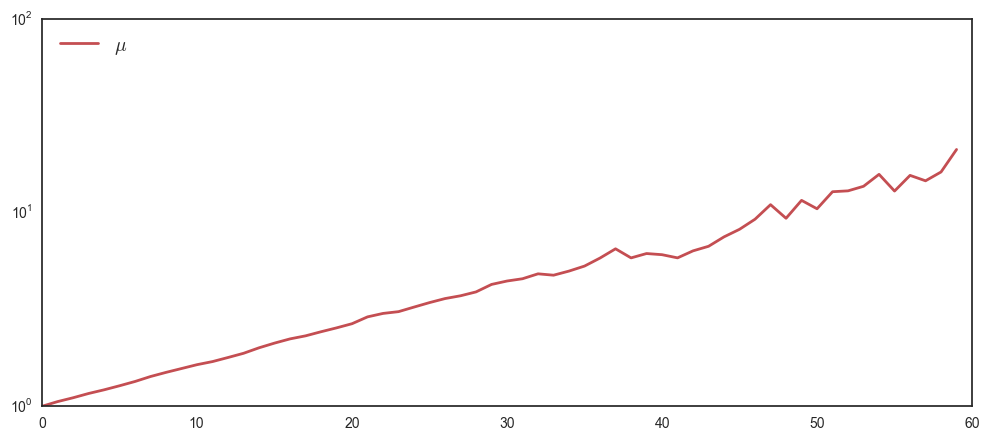
It seems like the empirical average \(\mu\) steadily increases. If you feel like removing more noise, you can increase \(N\) (however this script is quite slow due to all the for-loops).
As we have explicit knowledge of the dynamics, we can do much better than simulations. We can simply calculate the mean or expectation operator \(\mathbb{E}(\cdot)\) over the \(N\) trajectories. Formally, the expectation operator is the large-N limit of the empirical mean
\[\underset{N\rightarrow\infty}{\mbox{lim}}\left\langle W\right\rangle _{N}=\frac{1}{N}\sum_{i=1}^{N}W_i(t)\]where \(\left\langle W\right\rangle _{N}\) denotes the average over N, as N goes to infinity. We denote this \(\mathbb{E}\).
Let’s calculate this. By using our knowledge that as \(N\rightarrow\infty\) the probability of a fair coin asymptotes to the same ratio. This means we can calculate \(\mathbb{E}\) as \(\frac12\times0.6+\frac12\times1.5=1.05\) which is a number larger than one, reflecting positive growth of the ensemble of trajectories.
Below is a graphical result of the expectation operator \(\mathbb{E}\) and the empirical mean (\(\mu\) for a finite N).
interact(multiplicativeW, T = 60, N = 10000, W = False, E = True, A = False, mu = True)
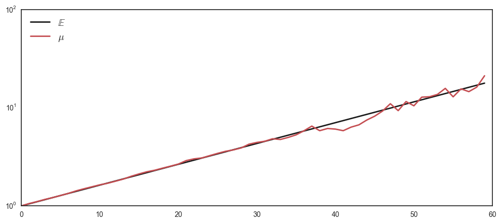
The graph supports our theoretical analysis: The empirical mean seems to asymptote to the large-N limit mean, which grows exponentially towards infinity.
The conclusion is simple: Since this process has a positive expectation it will simply grow exponentially towards infinity, which means that you (or anyone rational) should be willing to pay any ticket price P for playing this gamble.
Sounds too good to be true? Well, thats because it is too good to be true. To understand why, we must first consider the time-perspective.
The time-perspective
To convince ourselves about this, lets plot one ‘person’ \(N=1\) playing the game for \(T=10000\) trials and contrast this to the expectation operator \(\mathbb{E}\).
interact(multiplicativeW, T = 10000, N = 1, W = True, E = True, A = False, mu = False)
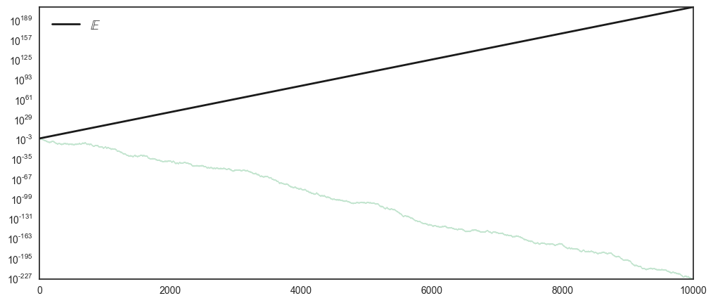
This single trajectory is quite a different scenario from what the theoretical prediction. While the expectation operator goes to \(10^{189}\) (which is a very, very large number), the realised trajectory ends up at \(10^{-227}\).
Let’s try to convince ourselves that this was just one unlucky trajectory. Again, we wish to remove noise, and we do so by increasing the number of players, playing \(T=10000\) to \(N=100\).
interact(multiplicativeW, T = 10000, N = 100, W = True, E = True, A = False, mu = False)

Immediatly there seems to be a fundamental difference between the theoretical prediction \(\mathbb{E}(\cdot)\) and the hundred realised trajectories.
Lets consider the definition of the finite-time time-average
\[\left\langle W(t)\right\rangle _{T} = \frac{1}{T}\sum_{t=0}^{T}W(t)\]Where \(\left\langle W(t)\right\rangle _{T}\) denotes the average of a single process over time \(T\). This quantity evolves over time as shown in the figure below. Similar to the above, taking the time-limit of this gives us the infinite time-average
\[\underset{T\rightarrow\infty}{\mbox{lim}}\left\langle W(t)\right\rangle _{T} = \frac{1}{T}\sum_{t=0}^{T}W(t)\]If we calculate this for the above dynamics, we will realise that it asymptotes to zero. The calculation is easy \(\sqrt{1.5\cdot0.6}\approx0.95\), a number less than one, indicating negative asymptotic growth.
Thus we have the two fundamental results that in the above scenario
\[\underset{T\rightarrow\infty}{\mbox{lim}}\left\langle W(t)\right\rangle _{T} \rightarrow 0\] \[\underset{N\rightarrow\infty}{\mbox{lim}}\left\langle W\right\rangle _{N} \rightarrow \infty\]This difference can be explained by considering a rough definition of ergodicity:
A process is non-ergodic if the time-average does not equal the ensemble-average.
That, formally can be expressed as
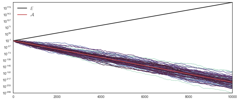
\[\underset{T\rightarrow\infty}{\mbox{lim}}\left\langle W(t)\right\rangle _{T} \neq \underset{N\rightarrow\infty}{\mbox{lim}}\left\langle W\right\rangle _{N}\]Plotting the finite ensemble and time-average will hints towards this difference being palpable in finite time as \(\mathcal{A}\) goes to zero, while \(\mathbb{E}\) goes towards infinity.
interact(multiplicativeW, T = 10000, N = 100, W = True, E = True, A = True, mu = False)
There’s much more to this story, and if you find it compellin, I suggest you see the video in the introduction, or read the follow papers: